Post description

In this post I wanted to recollect and consolidate my experience performing bayesian inference, in the particular case of a linear model under sparsity assumptions when the number of observations is much lower than the number of parameters. Emphasizing the practical difficulties that I found, and the philosophical questions that arose along the way. I’ll work over a synthetic dataset that aims to replicate the materials design problem that motivated the post , when we have many molecular descriptors as predictors and few observations, and we’d like to propose new candidates to test in the lab, so uncertainty estimation is an essential part of the solution. Similar problems are found as well in gene expression identification scenarios.

Code and Collab notebook (very slow).

Introduction

Trying to model the distribution $P(y|x)$ of the variable $y$, if we assume linear responses in a model and normal errors, $Y = X\beta+\epsilon$, the maximum likelihood estimation of our parametrized distribution $P_{\beta}(y|x)$, will lead us to the nice and home-like least squares problem, with a closed solution given by

$$ \beta = (X^{T}X)^{-1}X^{T}Y $$

Where X is the $N_{samples} \times N_{features}$ data matrix. When we have more samples than predictors $(X^{T}X)^{-1}$ is not defined, there is no unique solution anymore, there are infinite combinations that can perfectly fit the data points. In practice we can include our knowledge and experience about the nature of the generating data distribution to restrict weights or regularize the parameter space of possible solutions. In the maximum likelihood setting, this is in practice done with a penalty term in the cost function in the like the following one

$$ Loss = \sum_{data}(y-X\beta)+\lambda \sum_{i}|\beta_{i}| $$

The penalty strength, controlled by $\lambda$, will trade variance in exchange of bias. In the case of shrinkage penalties like L1 or L2, we are orienting the parameters toward small values, this is justified by characteristics that will most likely be present on our dataset; we know the magnitude of possible responses, and we know that weak predictors or small variance noise signals will inflate their coefficients to compensate their lack of correlation. We could reasonably expect as well, that a small number of predictors will dominate the, variance of the response variable, so we could encourage more parsimonious models.

Now, how do we get estimates of our uncertainty in these cases? We are including a bias based on our beliefs about the system, and there isn’t a systematic way of incorporating this within a frequentist analysis. We could resort to heuristic ad-hoc methods like selecting a subset of the strongest predictors and calculate confidence intervals for them.

We might resort as well, to bootstrapping and data splitting methods where we sample from the data distribution and observe the variability of the estimators fitted on different subsets of the data, knowing that as the number of samples increase, the values will converge to the population distribution values.

This is easy, fast, and hence popular, but in the regime of very small number of data points, if we split the dataset in non overlapping subsets, we will be increasing greatly the variance of the estimators, and, on the contrary, if the subsets overlap, there will be strong correlation between samples that shrink variances and give overconfident predictions¹.

This strategies might work well, and they are complementary to other approaches, but it won’t take long before we need peace and spiritual completitude by getting uncertainty estimates on a more principled basis that adhere with the beliefs incorporated.

Here is where Bayesian inference come to play. We get rid of the frequentist idea of the true value of a parameter, that we'd get for instance by finding the ML estimate of $P(\theta|y,x)$ over all population data , and instead use bayes formula to sample from the posterior distribution $P(\theta|y,x) \sim P(y|x,\theta)P(\theta)$, where $P(\theta)$ encompasses our prior belief on the parameters.

Problem description

The problem I’ll use as guide, will be the following weak sparse regression problem, where the coefficients come from two populations. One dominant population of $N_{w}$ weak predictors, and a much smaller population $N_{s}$ of strong predictors.

$$ \begin{array}{l} Y=X\beta^{T}+\epsilon \\ \epsilon \sim \mathcal{N}(0,5e-2) \\ N_{w} \quad coefficients \quad \beta_{small}\sim \mathcal{N}(0,1e-2)\\ N_{s} \quad coefficients \quad \beta_{relevant}\sim \mathcal{N}(0,1),\beta_{1} = 0.9, \beta_{2} = 2.1\\ N_{s} = 2 <<N_{s} = 200 \\ n_{samples} = 20<<p_{predictors} = 202 \end{array} $$

Selecting the prior, sparsity inducing distributions

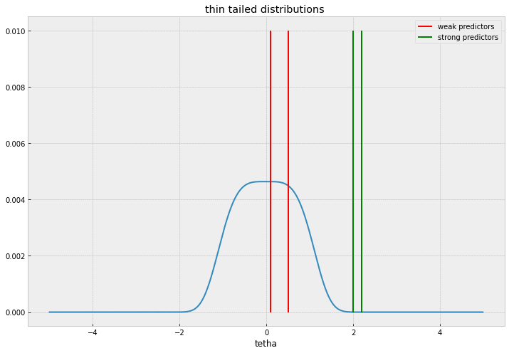
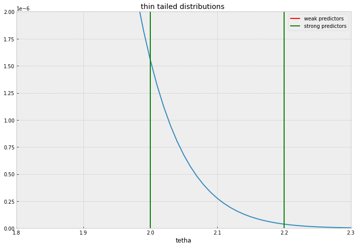
We need a prior distribution $P(\theta)$ that weights down the probability $P(\theta|y,x) \sim P(y|x,\theta )P(\theta )$ for small values of $\theta$ that accompany weak predictors, and encourage parsimony explanations of the variance, without biasing down the larger values of the predictors with strong responses.

Ideally, we should be looking for a fat tailed distribution that accomodates large values without relative penalty but at the same time accumulates mass sharply near 0.

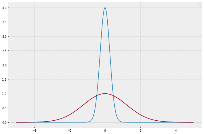
The Normal distribution ( Ridge regression equivalent in ML estimation), won’t be a good candidate because it will shrink everything alike without discrimination, the behaviour of thin and fat tailed distributions is illustrated in the plots below.

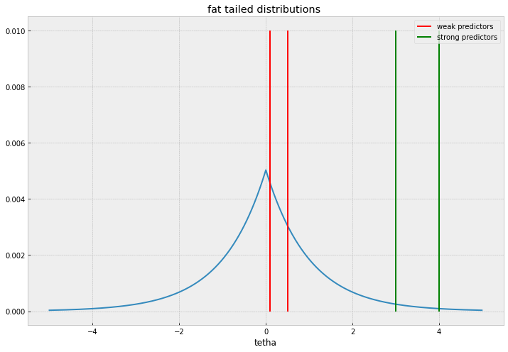
There is a big relative difference of weights in thin-tailed distributions around the origin, which, at the same level of variance explanation, promotes sparse solutions. Conversely, there is no much relative difference in weights for large values, what makes the pull around the origin stronger. This is reversed for fat-tailed distributions We have to keep in mind that we'll use a product of independent distributions as prior for the parameters, so parsimony will be enforced when a lot of parameters that are in low density regions of the prior are needed to fit the data, conversely, the great increase in likelihood will overcome the penalty induced to small groups of coefficients that explain a lot of variance.

I’ll comment two common distributions used, Laplace distribution , and Spike and slab distributions. Laplace priors and its ML estimation cousin, the Lasso regression is the workhorse for sparse regression, given its simplicity and familiarity.

$$ P(\theta|y,x) \sim \mathcal{N}(y-X\beta, \sigma)\frac{1}{2b}e^(-\frac{x}{b})$$

It’s like the “braveheart” of sparsity inducing distributions, it is overly-simplistic, it doesn’t represent the most accurate description of events, returns heavily biased impressions of coefficients and scottish medieval military logistics and underestimates the lethality of an english cavalry charge, but strike me blind if you would not totally recommend it to a friend.

Spike and Slab priors consist of a mixture of a thin distribution and a width one, commonly normal distributions are chosen. This priors captures more accurately the parameter distribution that arises in this kind of problems, where we have 2 distinct categories of predictors, strong predictors that appear in a ratio $p_{s} = \frac{N_{s}}{N_{total}}$ and, weak predictors, with ratio $p_{w} = \frac{N_{w}}{N_total}$, usually with $p_{s}<<p_{w}$.

$$ P(\theta|y,x) \sim \mathcal{N}(y-X\beta, \sigma)(p_{s}\mathcal{N}(\beta, \sigma_{s})+p_{w}\mathcal{N}(\beta, \sigma_{w}))$$

Selecting prior hyperparameters to reflect our prior beliefs

One of the strengths that are often highlighted about bayesian methods is that they offer a natural way to incorporate our previous knowledge about the system and then reason about the results. For this to be useful, the prior distribution must capture as faithfully as possible our prior belief about the parameters, which is not a trivial or easy task. For instance a phD on statistics might suggest us a very cool and complex distribution that works well for a specific problem, but if we don’t really understand the assumptions we are making with that distribution, we don’t really know which hypothesis the results are really reinforcing/invalidating.

What knowledge we want to incorporate about this model?

It is reasonable to have a gross estimate on the expected variance of the residuals, for instance, the repeatability and resolution of physical measurements, will constitute a lower bound for the expected deviation, we must include this to inform the model that explaining the variance beyond this limit is not significant. We might have as well an idea of the number of strong active predictors, or the span of admissible values for the responses. We could think of a threshold of significancy for the values of the coefficients, we can peek at the data, tinker with maximum likelihood sparse regression estimates etc. so we can delimit a range for parameters values that we feel comfortable with.

The more we don’t know, the bigger and less informative this ranges will be, and the more data we’ll need, to be able to extract significantly statistical conclusions from the results.

For this problem at hand, there are some few simple derivations that will give us plenty of insight to guide the confection of the model.

On the limit of a very large number of variables, assuming independent standardized predictors, the variance of $y$ will be

$$\sigma_{y}^{2} = E((X\beta+\epsilon)^{2})-E((X\beta+\epsilon))^{2} = \sigma_{\epsilon}^{2} + N_{w}\sigma_{\beta_{W}}^{2}+ \sum_{N_{s}}\sigma_{\beta_{S}}^{2}$$

so the expected variance of the residuals will be

$$\sigma_{res}^{2} = \sigma_{\epsilon}^{2} + N_{var}\sigma_{\beta_{W}}^{2}$$

Now, if we knew which subset of predictors were significant a priori, we could consider all the rest of weak predictors as added gaussian noise, and calculate the covariance of the strong predictors coefficients estimates

$$ cov(\beta) = E ( \beta\beta^{T}) = E( (X^{T}X)^{-1}X^{T}Y) (X^{T}X)^{-1}X^{T}Y)^{T}) = $$ $$ ((X^{T}X)^{-1}\sigma_{res}^{2}) = \frac{\sigma_{\epsilon}^{2} + N_{var}\sigma_{\beta_{W}}^{2}}{Nsamples} $$

This last formula will serve as an estimate of the resolution/identifiability we might expect on the model parameters.

Models and experiments

Laplace prior

The most basic probabilistic model $P(y|\theta,X)P(\theta)$ with a laplace prior can be expressed as this:

$$ \beta \sim e^-|\beta|/b $$ $$ \sigma_{y} \sim \mathcal{U}(\sigma_{min}, \sigma_{max}) $$ $$ y \sim \mathcal{N}(X\beta,\sigma_{y}) $$

Along with the data points, this would be enough to directly transcribe it to a bayesian inference framework syntax, in this case pymc, so it can sample from $P(\theta|y,x)$ by Markov-chain-montecarling the heck out of $P(y|\theta,X)P(\theta)$.

model = pm.Model()

with model:

    beta = pm.Laplace('beta',0,b, shape = (len(X[0])))
    ymu = pm.math.dot(X,beta)

    ysigma = pm.Uniform('ysigma',sigmin,sigmax)
    ys = pm.Normal("Y",ymu,ysigma,observed = y)
    idata = pm.sample(1000, tune = 500, cores = 12)

Now, let’s estimate the hyperparameter and refine it a little bit.

There are many things we can do to pin down a value for b.

We could, without much trouble, come up with a significancy threshold for the weak predictors, $\sigma_{W}$, and if we want the Laplace prior to pull to zero everything below that, we can equate the Laplace distribution variance to this threshold:

$$ 2b^{2} = \sigma_{W}^{2} $$

We can as well get a gross estimate of $b$ by doing a maximum likelihood cross validated lasso regression.

In the same spirit of last section we can gain a lot of insight by working on the limit of very large number of independent predictors.

Let’s write the log probability of our model

$$\sigma_{res}^{2} = \sigma_{\epsilon}^{2}+N_{var}\sigma_{\beta}^2 \approx N_{var}\sigma_{\beta}^2$$ $$-log(P)=ctte-N_{samples}ln(N_{var}\sigma_{\beta}^2)+\sum^{N_{samples}}\frac{(y_{n}-X_{n}\beta)^{2}}{\sigma_{res}}+\sum^{Nvar}{\frac{|\beta_{i}|}{b}}$$ $$-log(P)=ctte-N_{samples}ln(N_{var}\sigma_{\beta}^2)+\sum^{N_{samples}}\frac{(y_{n}-X_{n}\beta)^{2}}{N_{var}\sigma_{\beta}^2}+\sum^{Nvar}{\frac{|\beta_{i}|}{b}}$$

Now, we want to prevent weak predictors to spuriously fit single data points: If we single out any random $\beta_{i}$, because there is going to be a lot of $\beta_{j}X_{j}$ that are statistically independent, their sum is going to be near zero, so we could move that $\beta_{i}$ to fit a single data point, and repeat the process for the rest of the samples to perfectly fit them. Therefore, we should aim for the prior term on the right, to be somewhat larger than the loglikelihood gained per perfectly fit sample, this is going to punish predictors that explain few samples, but for the strong predictors that on their own explain the variance of many samples, we want the log normal term to dominate.

$$-log(P)=ctte-N_{samples}ln(N_{var}\sigma_{\beta}^2)+\sum^{N_{samples}}\frac{(\sigma_{y}-\beta)^{2}}{N_{var}\sigma_{\beta}^2}+\sum^{Nvar}{\frac{|\beta_{i}|}{b}}$$

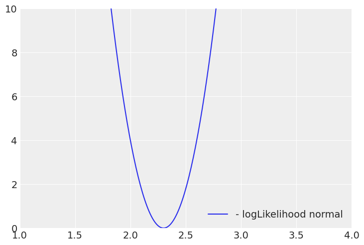
Plotting the per sample loglikelihood for a single coefficient:

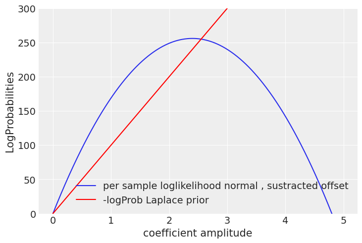
When the red line crosses the normal log likelihood, the prior will dominate and prevent a single coefficient going beyond that point, we don’t want to bias excessively strong predictors, but that depends as well on how conservative we want to be, like in life ,the more strong your prior beliefs are, the more evidence you will need to change your mind, that’s why it’d take many more good mad max reboot sequels before I could consider them to be a worthy competitor of the mesmerizing Tina Turner dancing moves on the 1985 sempiternal classic, Mad Max Beyond Thunderdome, a post-apocalyptic city fueled by pig manure, with a dwarf major whose worse nightmare is being eaten by the hogs underground, WOW!

So, with all of this, We could suggest reasonable values of $b$ but We probably couldn’t attribute any special meaning to one in particular, so the most appropriate thing would be to reflect that uncertainty on the model, with a uniform prior on $b$.

$$b \sim \mathcal{U}(bmin,bmax)$$

We might have a more or less precise knowledge of $\sigma_{res}$, but nevertheless, with very few samples, there is going to be a very high variability associated to the discrepancies between sampling and population distributions.

The sampling variance follows a $\chi^{2}$ distribution that quantify its probability deviation from the population value.

$$ (N_{samples}-1)\frac{\hat{\sigma}^{2}_{res}} {\sigma^{2}_{res}} \sim \chi^{2}$$

Even if we knew the population variance, for a sample size of 20, we could easily get variances in the +-50% range.

With all this, the model at hand will be:

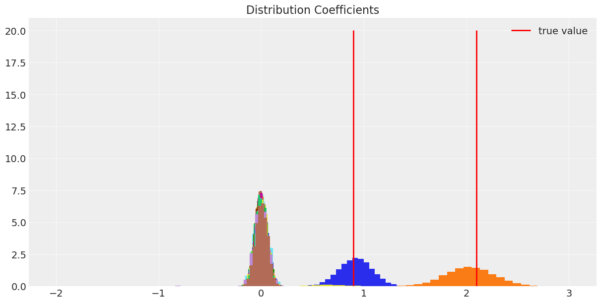
$$ b \sim \mathcal{U}(bmin,bmax) $$ $$ \beta \sim e^{-|\beta|/b} $$ $$ \sigma_{y}^{2} \sim \mathcal{\chi^{2}}\sigma_{res}^{2}/(N_{samples}-1)\ $$ $$ y \sim \mathcal{N}(X\beta,\sigma_{y}) $$

I’ll compare the results with the distribution of coefficients we get by doing maximum likelihood Lasso regression on draws of $N_{samples}$ tested against a fixed large sample size.

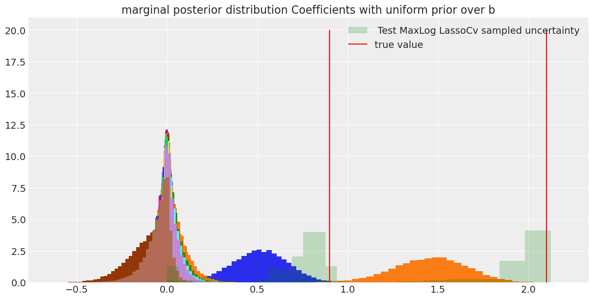
First picture marginal distributions of the coefficients for the population sampled cv lasso, and for the bayesian model. Middle image bottom image, Ypred Y test for lasso and for bayes with 20 and 12 samples respectively.

Comparing with the cv lasso we can see that our coverage was quite conservative, but allows us to discriminate the significant response of the predictors with a quantifiable certainty. On the other hand, on a single draw of the cv lasso we could have gotten a wide range of coefficients and we would really know how to trust them.

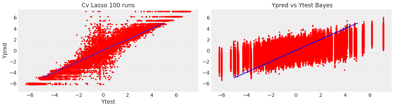
Comparing the predictions for the test data with 20 a and 12 samples, the differences between bayesian inference and ML estimation are manifest. The CVlasso estimates are guided by the data exclusively, so , with very small sample sizes it will have a larger variance, but it will give unbiased estimates. On the other hand the variance of the bayes model increases slightly , so it is more robust, in exchange for more bias, because instead of the sample distribution, is our previous belief which dominates in this scarce data regime. This is a clear example of the bias-variance trade-off.

I think this example , makes clear, what is , for me one of the most powerful points about bayesian inference, it provides us with a framework to answer, on a principled basis, questions like, “How much data will I need?”, “What is the minimum batch size of samples I’ll need to provide an informative answer”? Within the bayesian approach, every data point will add some information that will increase our confidence in a measurable way.

Spike and Slab prior

In the last section, we got very conservatives estimates in part because it was not straightforward quantifying our prior beliefs with laplace priors.

With a thin-fat gaussian mixture prior, besides promoting sparsity, we can naturally accommodate the categorical quality of strong/weak predictors, so we can capture our beliefs without involved analysis.

Let’s write down the basic model

$$ c_{i} \sim Bernoulli(p_{inclusion}) $$ $$ \beta \sim \mathcal{N}(0,\sigma(c_{i}))$$ $$ \sigma_{y}^{2} \sim \mathcal{\chi^{2}}\sigma_{res}^{2}/(N_{samples}-1)\ $$ $$ y \sim \mathcal{N}(X\beta,\sigma_{y}) $$

Now there is an extra parameter per variable adding some extra complexity , the inclusion probability $p_{inclusion})$, which on the contrary to the Laplace global shrinkage parameter \(b)\, will give the model extra flexibility to avoid biasing down large coefficients while pulling weaker ones towards 0.

The sizes of the thin and fat normals should match the magnitude of the expected responses for weak and strongs predictors, that we can assume we’ll be able to bound to some extent. While the $\sigma_{W}$ for weak predictors used in the experiment is 1e-2, there are some numerical issues having a mixture of two gaussians with very different variances, for very small sample sizes, when the prior has a very large effect on the posterior landscape, it creates a “stiff” problem for the hamiltonian montecarlo integration steps. There are reparametrization options that aide in this regard, but the least annoying solution for me is being a little more conservative and increase the size of the thin distribution until the divergences in the sampling process decrease to a reasonable amount.

Adding the tweaks with the $\chi^{2}$ commented in the last section, and given reasonable prior uniform intervals for the inclusion probability ( in the experiment, only 1% of the variables are strong predictors), the implementation in pymc would be the following:

sigma_thin = 6e-2
sigma_fat = 3
model = pm.Model()

with model:

    pinclusion = pm.Uniform("pinclusion",0.0,0.07)
    inclusion = pm.Bernoulli("bernoulli",pinclusion, shape = (nvars))

    beta = pm.Normal("beta",mu=0, sigma = (1-inclusion)*sigma_thin+inclusion*sigma_fat)


    ymu = pm.math.dot(X,beta)
    ysigma = pm.ChiSquared("chi",samples-1)
    ysigma =ysigma*(nvars*beta_sigma**2+sigma**2)/(samples-1)
    ysigma = pm.Deterministic("sigma",np.sqrt(ysigma))
    y = pm.Normal("Y",ymu,ysigma,observed = Ydata)
    idata = pm.sample(3000, tune = 1000, cores = 12,target_accept = 0.8)

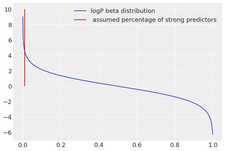
The problem with the last implementation, is that hamiltonian monte carlo samplers, the default MCMC method in most libraries, because of its superior performance on high dimensions, exploit the distributions gradient information, so they need to be differentiable. With a discrete Bernoulli distribution, different solvers use different strategies, like, combining metropolis with HMC, or marginalizing the discrete variables, either way , when the number of variables increase, it can become pretty slow, so there is an alternative reparametrization, that uses a Beta(especial unidimensional case of the Dirichlet distribution) distribution to overcome this issue.

$$ p_{inclusion} \sim Beta(\alpha,\beta) $$ $$ \beta \sim (1-p_{inclusion})\mathcal{N}(0,\sigma_{W})+p_{inclusion}\mathcal{N}(0,\sigma_{S})$$ $$ \sigma_{y} \sim \mathcal{\chi^{2}}\sigma_{res}/(N_{samples}-1) $$ $$ y \sim \mathcal{N}(X\beta,\sigma_{y}) $$

We can think of the Beta distribution as a “soft” Bernoulli, where the expected probability will be given by the ratio $\frac{\alpha}{\alpha+\beta}$, and the variance will decrease somehow with the magnitud of the vector $(\alpha,\beta)$. So, with $\alpha,\beta \rightarrow \inf$ the distribution will tend towards a Bernoulli distribution with probability $\frac{\alpha}{\alpha+\beta}$.

I personally tune this “level of softness” in two ways, increasing it until I start to get a lot of divergences and then in a similar way as I did with the Laplace pior. Comparing the log-probability of the beta distribution with the log-likelihood per sample in the limit of large variables.

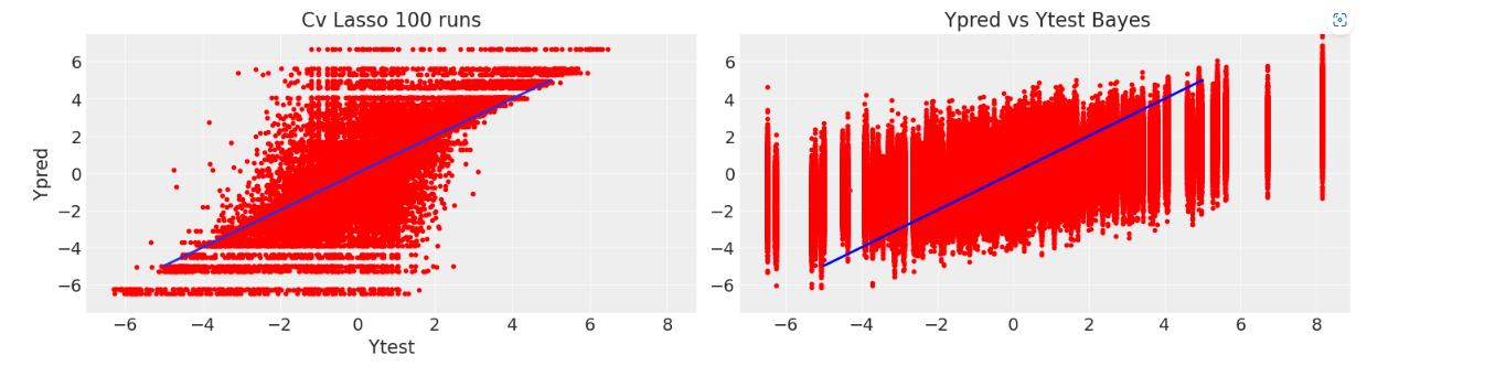
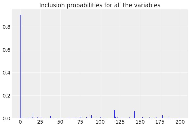
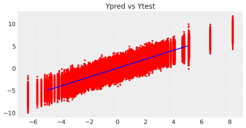
As shown in the plots below, now the model directly gives us , the inclusion probability for each variable. Checking the Ypred vs Ytest graphic and the marginal distributions for the coefficients, it is clear that the model is way less biased, because it is closer to the generating distribution.

Other sparsity inducing distributions, Horseshoe distribution

Another popular choice of sparsity inducing prior distribution introduced in ², is the Horseshoe distribution, which has not an analytical expression, but can be easily defined as a hierarchical model:

$$ \beta_{m} \sim \mathcal{N}(0,\tau\times\lambda_{m})$$ $$ \lambda_{m} \sim Half-\mathcal{C}(0,1) $$ $$ \tau \sim \sim Half-\mathcal{C}(0,\tau_{o})$$

In the same way as the gaussian-mixture model, it uses an extra parameter per predictor $\lambda_{m}$ to allow custom shrinkage, and a global shrinkage parameter $\tau$. These parameters are sampled from fat-tailed Cauchy distributions, with a polynomial decreasing rate, which might be excessively long-tailed, so there is another popular version of the distribution that is called Regularized Horseshoe ³.

It is a relatively new distribution, so, its theoretical properties, and proper numerical implementations are not as mature as the other priors used in the last sections. With a little digging online various reports about the burden that it imposes on the HMC sampler can be found, and by all that is nice and beautiful on this earth, I could not make the sampler converge for the specific study case , anyway, it is in the associated notebook so you are welcome to try it.

Thus, I won’t extend further, there is a more detailed explanation in ⁴.

Conclusions

The ability to include domain knowledge into the inference problem, is one of the mantras used to promote bayesian methods, and, albeit this is one of the most enticing features about them, its practical realization might be far from trivial.

I think that frequentist and bayesian method can work in tandem and complement each other well. The variance of cross validation and bootstrapping estimations, exclusively data guided, decreases rather rapidly with the sample size, so they may constitute an useful assistance in bayesian inference to perform sanity checks and hyperparameter estimation. On the other hand, frequentist analysis give full coverage under certain assumptions, and that can be leveraged into our distribution to have more robust estimates

Even if we have our model perfectly defined, matching nicely our prior beliefs, we may run into numerical issues in the sampling process that make the approach unfeasible, which would require non trivial reparametrizations to fix it, or a solid understanding of the monte-carlo samplers, which might contribute to specialize the application of this methods.

Beyond all of its caveats, the ability to incorporate very small batches of samples in a rigorous and consistent way that capture our prior assumptions, makes bayesian methods, in my opinion, one of the most, if not the most, enticing approachs to guide sequential problems that imply carrying out expensive evaluations or simulations.

Bayesian Sparse Regression: A practitioner experience