Deep Learning for PDEs: Fourier Neural Operator and Phase Field models
Introduction
In this post, I try to summarize the motivation and general idea behind learning PDEs from data with Neural Networks. I’ll support this by reporting as well, the results of applying some of the latest advancements in the field [Yuying Liu et al., 2020], [Zongyi Li et al., 2020] to learn the spinal decomposition dynamics described by the \(2D\) evolutive Allen-Cahn equation.
\[\begin{array}{l} \partial_{t}u-M(\Delta u -\frac{1}{\epsilon^{2}}(u^{2}-1)u) = 0 \\ u,\nabla u |_{\partial \Omega} \quad periodic \\ u(0,x,y) = u_{0}(x,y)\\ x,y\in[0,1] \end{array}\]All the code can be found here.
Why Deep Learning and PDEs?
Partial differential equations are one of the most concise and useful ways we have for representing the rules that describe the behavior of a system. Once we find a PDE that model some phenomena, we have some sort of a set of differential Conway’s game of life rules of the system. Modelling a system this way, we are not only able to compute possible evolutions and responses, but we can apply as well the powerful apparatus of calculus to get a lot of insight about the general behavior of the system.
The heat equation, the hello world of PDEs
So, what’s the catch? Well, for real problems of certain size, they are very expensive to solve. In fact, a big fraction of the world HPC resources are devoted to solve airfoil boundary layers, making weather forecasts, solving Black-Scholes to predict the price of Dogecoin…
So, we want to solve them more efficiently. But how does deep learning come in to play here?
To answer this, it is specially enlightening to discuss some basic classic approach to deal with a certain kind of PDEs amenable to analytical treatment, linear PDEs. We’ll consider the specific example of the vibrations of a guitar string.
The most basic model to describe propagation and undulatory phenomena, from acoustics to electrodynamics, is the wave equation.
A PDE without initial and boundary conditions has infinite solutions, we need to specify them to formalize our problem. The string is fixed at its ends, with an initial condition given by the elongation produced with our thumb, and \(0\) initial velocity because we are releasing it.
To solve numerically this equation we first have to discretize things. If we only mesh the space with some stencil we are left with a system of ODEs \(\dot{u}=f(u)\) of the amplitude of the solution on that node. Instead of meshing the space, we can as well discretize the spatial part by expanding \(u\) in some finite basis \(u = \sum a_{k}(t)\phi_{k}\), with \(\phi_{k} \in\{\phi_{1}(x)...\phi_{n}(x)\}\) \(u = \sum a_{k}(t)\phi_{k}\), and we’d get another system of ODEs \(\dot{a}=f(a)\) for the amplitude of the projection onto each basis function. The thing is, once we choose a finite representation of the space , we’ll get a system of ordinary differential equations whose solution will be the amplitude of the coefficients of the different basis functions over time. Our goal now is to choose a finite basis \(\{\phi_{1}(x)...\phi_{n}(x)\}\) such that we can have a very good approximation of our system with the least amount of basis functions.
For linear systems such as the wave equation we can find this basis analytically ,by applying separation of variables and finding the eigenmodes of the associated Sturm-Liouville equation. Each element of this basis will be an harmonic mode, and being an eigenmode, it will be orthogonal to every other basis element.
\begin{equation} u(x,t) =\sum_{n} sin(n\pi x/L)(A_{n}cos(n \pi ct/L)) \end{equation}
The idea of optimal basis will eventually depend on our specific problem. As the eigenmodes are orthogonal to each other, each of the associated ODE comprising the system will be decoupled from the others. If we prefer to analyze it from a probabilistic standpoint, the elements of this basis are uncorrelated, and can be thought as the principal components.
Now, the projection of the initial shape of the string onto this basis will determine the coefficients \(A_{n}\), this is how much each harmonic is “stimulated”, and this is going to unambiguously specify the evolution of the system.
Keeping only the harmonics with more energy , we are going to have a good approximation of the string dynamics, if we pluck the string here or there, with more or less strength, we might need a few extra modes to meet a certain accuracy requirement, but in any case we can know the state of our system with way less parameters than if we worked on the original \(x_{i}\) discretization.
The key thing here is, the wave equation can describe a vast amount of behaviors in systems with different geometries or with much broader spectral responses, but in our specific applications, we are going to be using just a tiny subset of the space of possible solutions, the wave equation is like a compilation of maps for every museum of oscillatory phenomena , but if we are visiting a specific museum, we want a map of that building , not a cumbersome 5km x 5km chart that details every museum in the world.
Hopefully, the role of Deep Learning here begins to become clearer, what we really did back there was a coordinate transformation from the original representation of the PDE \(x\) to \(w\), the frequency domain. Instead of computing the amplitude of the solution over each \(x_{i}\) node \(U_{i}\), we compute the amplitude of the solution over each \(w_{n}\) mode, \(A_{n}\)
In the end, this was accomplished with a linear transformation that we can find systematically in the case of linear equations, but if we introduce now a small non linear term such as
this term is going to mix and couple our beloved eigenmodes together, new modes, not considered in the truncated basis will be born from combinations of the original ones, this will be exacerbated the most present the effect of the non-linearity is. The trajectories of non linear evolutive PDEs, wont live in a flat manifold being each dimension the amplitude over one of the elements of the basis, there is no superposition principle so we can not insert linear combinations of our basis \(A_{1}(t)\phi_1(x)+A_{2}\phi_2(x)\) and expect them to be a solution of the PDE, the trajectories of the non linear PDE will live in curved manifolds, with no general way of finding the non linear transformation that takes us from our original space to this curved latent manifold 3, 4.
Most likely, the deep learning guy at the end of the room, being too busy trying to come with a strange name for his next paper, wasn’t paying attention to any of this. But as soon as the key terms manifold, representations, non linear transformation, unknown change of basis, are scattered into the air, he’ll be on the floor, uncontrollably convulsing with excitement.

Well, we can not blame him, Deep Learning has proven to be an invaluable tool to learn arbitrarily complex functions by mapping the data into a manifold of much lower dimension than the original space, encoding semantic variations continuously in the coordinates of this latent space. If this works with music and images, it is expected to perform even better with mathematical entities that live in a continuous and smooth manifold as it is the case with the solution of PDEs.
Example applications
We have already commented that the biggest contribution of DL to PDEs problems relies on the reduction of time complexity. More specifically, this entails immediate benefits in certain areas :
Besides the reduction in computing time, there are other interesting applications of deep learning to the world of PDEs
There are a lot of applications in dynamical system theory and classical mechanics for example, where knowing the change of coordinates that transform our system into some "canonical system" might give us a lot of insight about them, such as conserved quantities, normal forms etc.
Fitting the parameters of our PDE to data, or coupling some unknown term to our model can be very cumbersome in a specific classical numerical simulation, but Deep Learning libraries makes the data assimilation problem much more easy to couple.
So, how do we do it, how do we solve PDEs with deep learning?
Two general approaches
-
Supervised learning approach: Sample data from the population of solutions, and make the neural network learn the mapping \(NN: parameter \rightarrow solution\). Bhattacharya, Kaushik, et al. Model reduction and neural networks for parametric pdes. arXiv preprint arXiv:2005.03180 (2020)..
-
Weighted residuals approach: Reparametrice \(N_{p}(y,\frac{\partial y}{\partial x},...) = 0\) with a neural network \(\hat{y}(x,\theta)\) and minimize the residues of the associated functional along with the BCs. M. Raissi, P. Perdikaris, G.E. Karniadakis, PINNS.
Problem statement and approach
The problem
We consider the PDE \(P\) with BC as a mapping \(\psi\) between function spaces where \(X\) is the parameter space and \(Y\) the solution space.
In order to learn the mapping, \(X\rightarrow y\) (X might be the initial conditions , boundary conditions, constitutive parameters… whatever), we must sample \(N\) (X,Y) pairs with a traditional solver and feed them to a model.
Nice and extended explanation here.
The approach
The most obvious model to learn this mapping is a Convolutional Neural Network, because it exploits the coherence and translational invariance present in the solutions of PDEs.
One of the main issues with this approach is the following. Remember how we were talking in the example of the wave equation of a basis set of functions \(\{ \phi_{1}(x)...\phi_{n}(x) \}\) to represent our solution? with the CNN approach, we’ll learn a mapping between the discrete spaces where \(X\) and \(Y\) will be represented, but this mapping will be completely dependent on the mesh used in our training data, what if we first project \(X\) into a known basis of our choice \(\{ \phi_{1}(x)...\phi_{n}(x) \}\), we learn the mapping there and project back to \(Y\), so if the discrete representation of \(X\) changes, by changing the resolution of the snapshots for instance, the error committed will only be the projection error onto \(\{ \phi_{1}(x)...\phi_{n}(x) \}\), that shouldn’t be too great if we use a robust basis and the discrete \(X\) representation still contains enough information to characterize an univocal mapping.
Not only that, we know that some basis, such as Fourier Series expansions, are very well suited to sparsely represent PDEs solutions, so it should be more appropriate to start from the frequency domain rather than the space of CNN transformations.
This clever approach was introduced in , as a new neural network architecture, coined as Neural operator, in particular when the frequency representation space is used, Fourier Neural Operator or FNO.
In Summary
\(F\) and \(G\) are the operators that project the data onto a discrete space. The symbol \(\varphi\) represent the mapping in the discrete space.
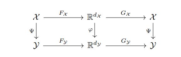
figure source
If we work directly in the discretized space, we’ll model the mapping with a convolutional neural network by minimizing:
\[\underset{\theta}{argmin} \underset{x \sim \mu}{E}(Cost(\varphi_{solver}(x)-\hat{\varphi}(x,\theta))\]If we work in a function space we’ll minimize:
\[\underset{\theta}{argmin} \underset{x \sim \mu}{E}(Cost(\psi_{solver}(x)-\hat{\psi}(x,\theta))\]Both methods work with discrete data , but in the first case , we are learning directly a mapping in \(R^{N_{grid}}\) while in the second case we first project the data onto a function space (Fourier Transform), we learn the mapping there and transform back to the discretized space.
Case study : Evolutive system, Allen Cahn, spinodal decomposition
I’ve evaluated FNO and CNN models in the specific problem of learning the dynamics of the Allen Cahn equation, a reaction diffusion system that models phase transitions, phenomena of coalescence, nucleation…
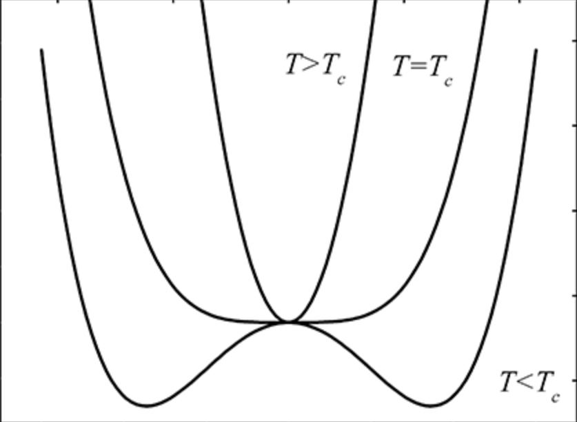
\[\begin{array}{l} \partial_{t}u-M(\Delta u -\frac{1}{\epsilon^{2}}(u^{2}-1)u) = 0 \\ u,\nabla u |_{\partial \Omega} \quad periodic \\ u(0,x,y) = u_{0}(x,y)\\ x,y\in[0,1]\times[0,1] \end{array}\]| Gibs free energy vs phase | Initial condition, small fluctuations that trigger the decomposition |
|---|---|
 |
 |
In the above equation \(u\) is the function that parametrize the phase of the system, with range \((-1,1)\)5.
Let’s imagine an isolated bottle full of water, under certain P,T conditions below the critical temperature, both gas and liquid water will coexist, while thermodynamics give us the equilibrium states, the dynamics of how we go from one state to another, is modelled by reaction diffusion systems like the Allen Cahn equation.
I am interested in the conditions that favor the coexistence of phases, where both liquid (1 phase ) and gas (-1 phase) are stable states, with a metastable state at 0.
We’ll start with a random small perturbation around the 0 metastable state that will evolve rapidly to form aggregates of continuous phase that evolve much more slowly.
| Simulations samples | \(M = 1,\epsilon = 0.01, T = 200 dt\) |
|---|---|
 |
 |
 |
 |
I find this a simple yet interesting test problem for various reasons. It is very easy to generate a diverse set of learning trajectories by just using white noise as the initial conditions. There is no chaotic behavior2 yet we have great sensitivity to initial conditions. The numerical integration of this equation constitutes a stiff problem, this means, it exhibits multiple spatial and temporal timescales that must be solved simultaneously to accurately predict long term behavior.
We have an extremely fast destabilization at the beginning, called nucleation that is followed by a slow evolution dictated by the interface between phases. Even if the coalescence stage is generally slow, when two drops are close to each other, they merge very quickly, a process that requires a small enough time step to be correctly captured.
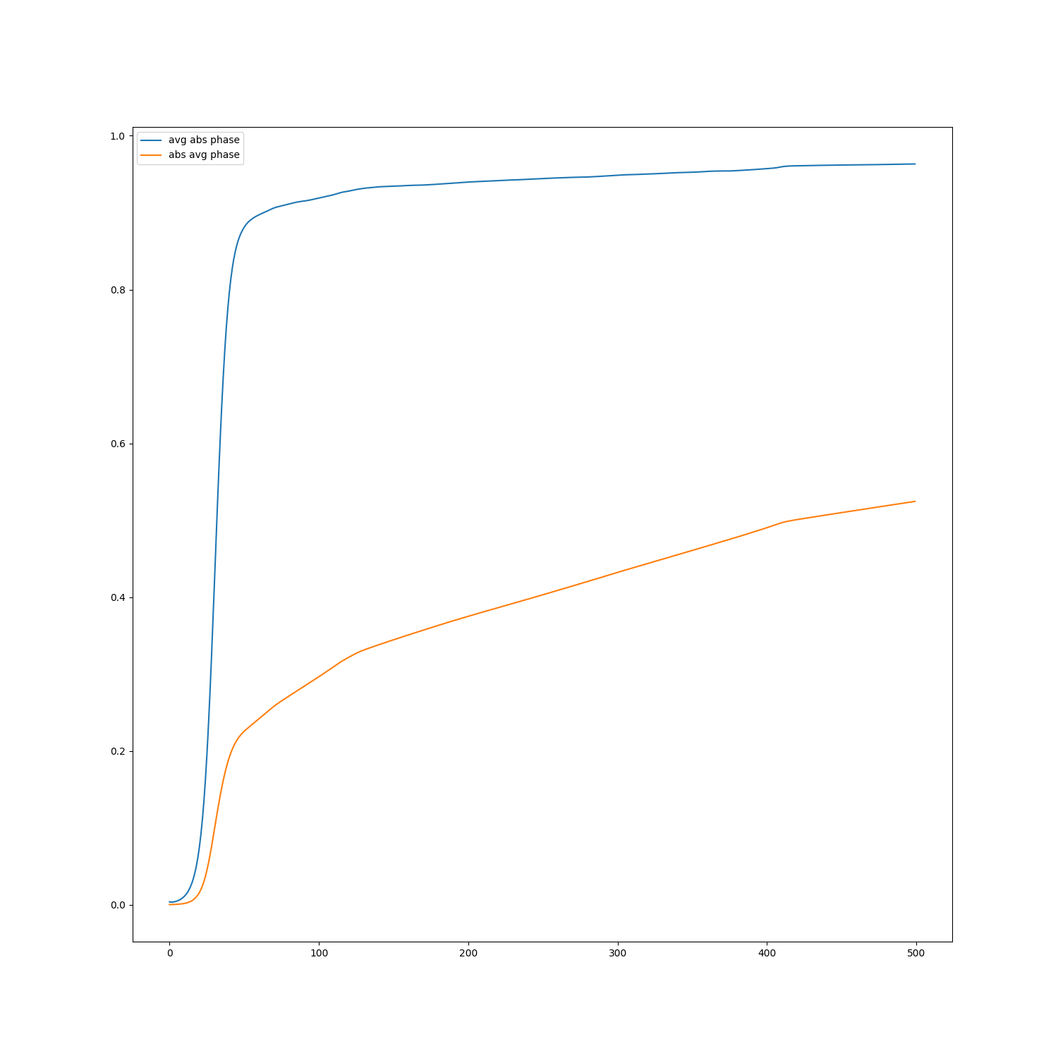
| time evolution | \(E(abs(phase))\quad vs \quad time\) |
|---|---|
 |
 |
Models architecture: CNN vs Fourier Neural Operator
The practical implementation of the method consists in what would be framed as an image-image regression problem in Deep Learning, such as denoising/enhancing problems, or semantic segmentation problems. The typical networks used in these problems are some variant of the U-Net architecture , a convolutional encoder decoder scheme with skip connections between symmetrical layers to enable the sharing of high frequency details along the network, so the latent space can encode more abstract features of the input.
| Image-Image CNN | Fourier Neural Operator |
|---|---|
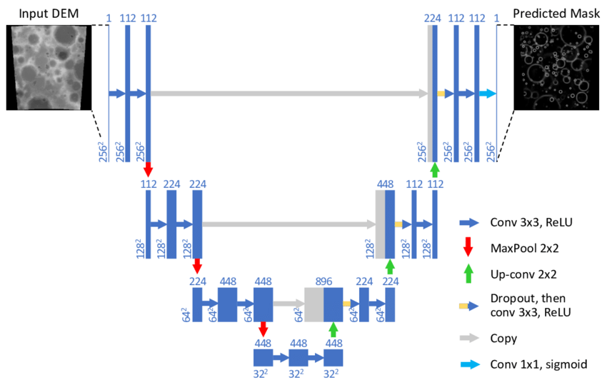 |
 |
While this is more of a conjecture of my own and it is not properly tested (as far as I know), I think implementing an aggressive bottleneck compression as the ones used in semantic segmentation is not necessarily beneficial. This is because in vision related domains, the semantic entities present in the input are invariant under a vast number of transformations of variable amplitude, you have to severely corrupt a picture of a cat so you can’t tell it is a cat anymore. This is an ideal setting for encoder decoder architectures to shine, because diffusive transformations are embedded in the inductive bias of these models. On the other hand, this is not the case with most PDEs, here the high frequency details might be very important and they might be entangled with the slow modes such as in stiff problems. Small differences in “pixel” space , can give rise to two completely different trajectories, such as in the case of the system we are studying , something that is not usually paralleled in vision domains.
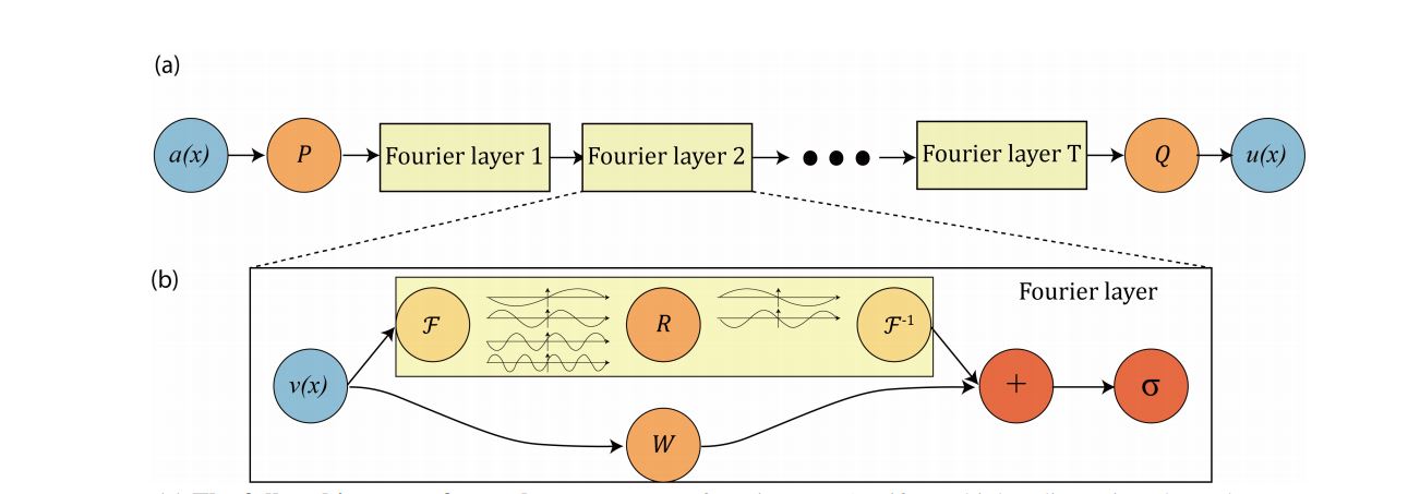
The Fourier Neural Operator is comprised of Fourier Layers as a drop-in replacement for convolutions. A (Channels,H,W) batch is forwarded to the Fourier Layer which applies a Fourier Transform, followed by truncation above a certain treshold frequency. Then a feed-forward-like mapping in the frequency domain follows and finally, the network state is translated back with an Inverse Fourier Transform to the (Channels,H,W) space, where it is summed via skip connection with a convolution applied to the input. The truncation of high frequency modes is a regularization mechanism that gives the network robustness to high frequency variations in the input space which are delegated to the traditional convolutional branch, which is needed besides, to enable the network to implement boundary conditions other than periodic.
Training and evaluation
The mapping we’ll try to learn is \(\Psi: u_{T-\Delta t}\rightarrow u_{T}\) aiming to later apply it recurrently to predict times much longer than \(\Delta t\), such as in [Yuying Liu et al., 2020]. As NNs operate in a different space than the original one, they’ll not be constrained necessarily by the time integration errors of traditional schemes [Yuying Liu et al., 2020], so larger prediction times can (and must) be used for long term prediction.
The loss function to minimize, the same used in [Zongyi Li et al., 2020] and [Yuying Liu et al., 2020], will be simply the square error of the prediction one step ahead and the ground truth snapshot.
\[\underset{\theta}{argmin}\underset{u_{0},T}{E}(|u_{T+\Delta t}-\hat{u}_{T+\Delta t}(\theta, u_{T})|^{2})\]We compute with Fenics 200 simulations with different random initial conditions sampled from \(N(0,\sigma = 0.2)\), we split them in a 140:60 training/validation dataset. For validation we skip the first steps so the initial noise is diffused and the emergence of patterns can be appreciated. An Backward Euler scheme was used to compute the solution, the first steps of the spinal decomposition required a smaller time step of \(dt/10\).
For training we use \(\Delta t = 6dt_{solver}\).
Results
FNO outperforms clearly the CNN, even though the later used many more parameters to obtain the same next step prediction accuracy. I wasn’t expecting the FNO to accurately reproduce all the simulation steps of a validation input just by training on the next step prediction, I was expecting to need some multi-scale multi-step approach to get this, (as it’d be required with the CNN) and was pleasantly surprised when it successfully reproduced the validation trajectories.
| FeniCS | FNO | CNN |
|---|---|---|
 |
 |
 |
 |
 |
 |
 |
 |
 |
Errors evolution in time
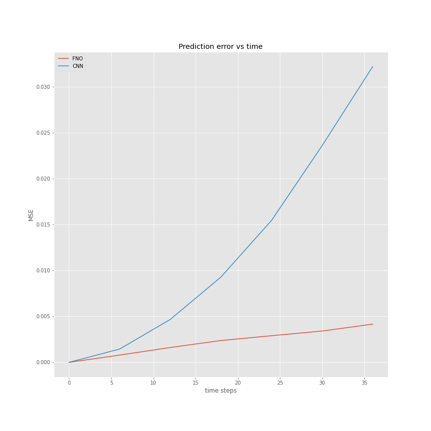
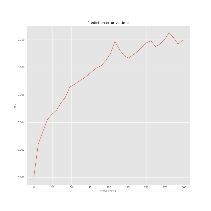
Comparison CNN vs FNO
Even if the long term stability of FNO was expected to be better than the CNN, both being trained up to the same error at the next time step prediction, FNO clearly outperforms the CNN model, an important contributing factor for this, is likely the recurrent projection onto the low frequency Fourier Layer which smooths artifacts and prevent them from accumulating error.
| CNN,FNO error vs time | FNO error time |
|---|---|
 |
 |
A key feature of both networks needed to obtain long term stability was the use of batch normalization, even if two twin networks, one with batch norm, and the other without, achieved the same next error prediction, the one without normalization exploded when applied recurrently.
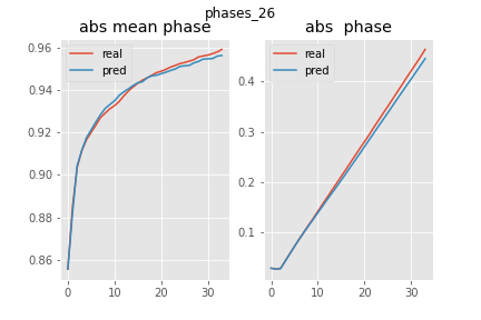
Evolution of macroscopic magnitudes
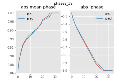
In the graphs below the pred vs real plots of the absolute mean phase \(E(abs(U))\) is showed, \(1-E(abs(U))\) is roughly the amount of interface present. As it is shown in the graphs below, this was accurately reproduced by the FNO.
| phase quantity vs time | 2D evolution |
|---|---|
 |
 |
 |
 |
Nucleation stage
Even if the initial nucleating phase was very short and consequently under-represented in the training dataset, the network, (which was trained with \(dt\) 60 times bigger than the ones needed for the Implicit Euler Scheme used in FeniCS to converge), surprisingly (magically even), it captures with fidelity most of the spinal decomposition from the initial random noise. There are some artifacts at the beginning, this is most likely because it must be mainly the convolutional part of the network the one providing the evolution of this high frequency fast initial dynamics, while the projection onto the Fourier modes space is very small. Once the patterns emerge the projection on the Fourier Layers starts to dominate and smoothens the evolution again.
It must be noted that the discrepancies that appear in cases such as the one in the middle, are explained by the FNO failing to capture the little bridge between the blobs of same phase, this leads to very different evolutions , even if the slow dynamics are well captured, is this kind of error trace which makes reaction diffusion systems such nice test problems.
Corrupted input
One of the great features of learning operators between functional spaces, is the great robustness they present to perturbations in the initial condition, that are projected back to the functional space of the Operator Layers.
| original | downsampled /2 | sampled 25% | Gaussian noise \(\sigma = 1\) |
|---|---|---|---|
 |
 |
 |
 |
 |
 |
 |
 |
This is specially useful if we are feeding the surrogate model with data sampled from sensors or corrupted with noise. If we were operating with the original equation, to reproduce the dynamics we should introduce a regularizing preprocessing step, such as interpolation or gaussian smoothing, here it comes in the pack. I didn’t report it here, but the same experiment with the CNN failed miserably ( and expectedly ) in reproducing the uncorrupted dynamics even with a smaller degree of perturbation.
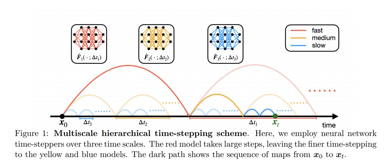
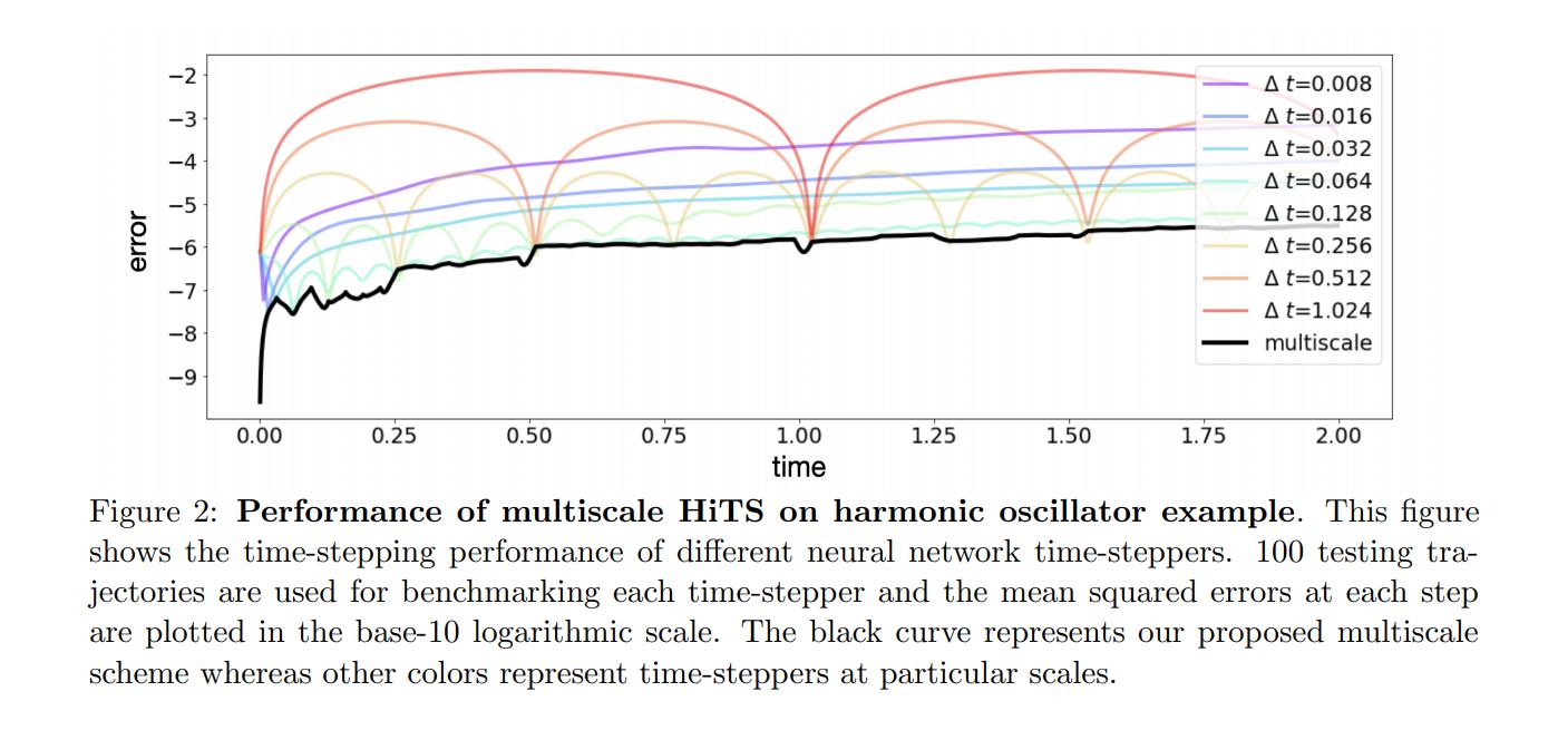
Multiple scales
As explained in [Yuying Liu et al., 2020] and [Raissi et al., 2018] very small steps leads to poor performance on the recurrent integration of the solution. NNs are sloppy learners that can not be expected to reach the low tolerances of classical multi-step schemes, the solution for long term integration is increasing the \(dt\) between samples at training time 3, allowing the network to overcome its lack of precision by sniffing what comes ahead and learning a coordinate transformation where time integration ( implicitly in the network) is easier. Nevertheless we might be interested in the solution of intermediate steps, for some real time feedback or if we want to appreciate every step of the morphing meme of Nicolas Cage after being used as initial condition in a reaction diffusion system.
Hierarchical Deep Learning of Multiscale Differential Equation Time-Steppers.
| Approach | different \(\Delta t\) errors comparison |
|---|---|
 |
 |
| \(2dt\) fourier network | \(12dt\) fourier network |
|---|---|
 |
 |
The evolution on the left is from a network trained on smaller timesteps , even though the big step network also misses some high frequency details( not so manifest in the training dataset, but essential to make Nick Cage such a trademark of great acting), doesn’t grow the artifacts that the small-step network present in the long term.
We can follow [Yuying Liu et al., 2020] and combine both time scales to achieve a fine evolution with long term accuracy
Some jumps are present when we switch to the big step network checkpoints, that could be corrected by introducing an intermediate time scale in between.
Footnotes
-
There is some special cases with known analytical transformation, such as the Hopf-Cole Transformation
-
With chaotic trajectories it is harder to understand the possible difficulties the network is experiencing, and there'll be separation of predicted and ground truth trajectories even the model learnt the dynamics perfectly.
-
This has limits, of course, in chaotic systems, if you exceed its Lyapunov time , there'll be a very small correlation, or no correlation at all, between \(u_{t}\) and \(u_{t+\Delta t}\)
-
For a more theoretical and traditional approach to this latent manifold thing, applied to dynamical systems, one of the key terms is Approximate inertial manifolds.
-
The range chosen to represent both phases is arbitrary, and depends on the domain of the two-well potential function we choose.
References
-
LI, Zongyi, et al. Fourier neural operator for parametric partial differential equations. arXiv preprint arXiv:2010.08895, 2020. https://arxiv.org/pdf/2010.08895.pdf?ref=mlnews
-
Holl, Philipp, Vladlen Koltun, and Nils Thuerey. Learning to control pdes with differentiable physics. arXiv preprint arXiv:2001.07457 (2020) https://arxiv.org/abs/2001.07457
-
Kim, Byungsoo, et al. Deep fluids: A generative network for parameterized fluid simulations. Computer Graphics Forum. Vol. 38. No. 2. 2019 https://arxiv.org/abs/1806.02071
-
Thuerey, Nils, et al. Deep learning methods for Reynolds-averaged Navier–Stokes simulations of airfoil flows. AIAA Journal 58.1 (2020): 25-36. https://arxiv.org/pdf/1810.08217.pdf
-
Lusch, Bethany, J. Nathan Kutz, and Steven L. Brunton. Deep learning for universal linear embeddings of nonlinear dynamics. Nature communications 9.1 (2018): 1-10. https://www.nature.com/articles/s41467-018-07210-0
-
Raissi, Maziar. Deep hidden physics models: Deep learning of nonlinear partial differential equations. The Journal of Machine Learning Research 19.1 (2018): 932-955. https://www.jmlr.org/papers/volume19/18-046.pdf
-
Liu, Yuying, J. Nathan Kutz, and Steven L. Brunton. Hierarchical Deep Learning of Multiscale Differential Equation Time-Steppers. arXiv preprint arXiv:2008.09768 (2020). https://arxiv.org/abs/2008.09768
-
Raissi, Maziar, Paris Perdikaris, and George Em Karniadakis. Multistep neural networks for data-driven discovery of nonlinear dynamical systems. arXiv preprint arXiv:1801.01236 (2018). https://arxiv.org/pdf/1801.01236.pdf
-
Bhattacharya, Kaushik, et al. Model reduction and neural networks for parametric pdes. arXiv preprint arXiv:2005.03180 (2020). https://arxiv.org/pdf/2005.03180.pdf
Acknowledgements
Among others, I’d like to thank Prashanth Nadukandi (a.k.a FEM Sandokan) for the thorough review of this post, and Ángel Rivero Jiménez for all the master classes on Phase-field models.